Model Diagnostics
In this lab we will work with the packages faraway and visdat. We will work with the data frame mammalsleep, from the faraway package. First, we load the data into our environment:
library(faraway)
library(visdat)
data(mammalsleep)
\(\require{color}\definecolor{teall}{RGB}{58, 171, 174} \definecolor{bluemoon}{RGB}{62, 71, 125}\definecolor{gween}{RGB}{73, 175, 129}\)
1. Find the best fitted model for predicting sleep.
a. Run a visdat analysis on the data:
We use the visdat package to visualize everything inside of the mammalsleep dataframe. From this plot, we can identify each variables’ class and whether the values are missing.
vis_dat(mammalsleep)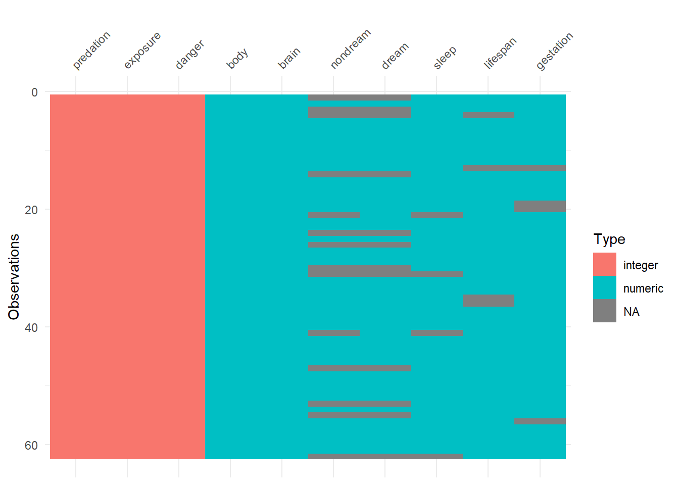
The visdat output shows the number of missing values for variables nondream, sleep, lifespan, and gestation.
b. Fit a squares regression model to predict Sleep:
Our dataset contains 62 observations, and we’ll use the following 7 variables in our model: body weight, brain weight, lifespan, gestation time, prediction index, sleep exposure index, and danger. But first, we remove observations with missing values for the outcome sleep and the predictors lifespan, or gestation.
df <- mammalsleep[(!is.na(mammalsleep$sleep) &
                     !is.na(mammalsleep$lifespan) &
                     !is.na(mammalsleep$gestation)),]
mod <- lm(sleep ~ body + brain + lifespan + gestation +
predation + exposure + danger,
data = df)
c. Test the model assumptions:
Constant Variance Assumption.
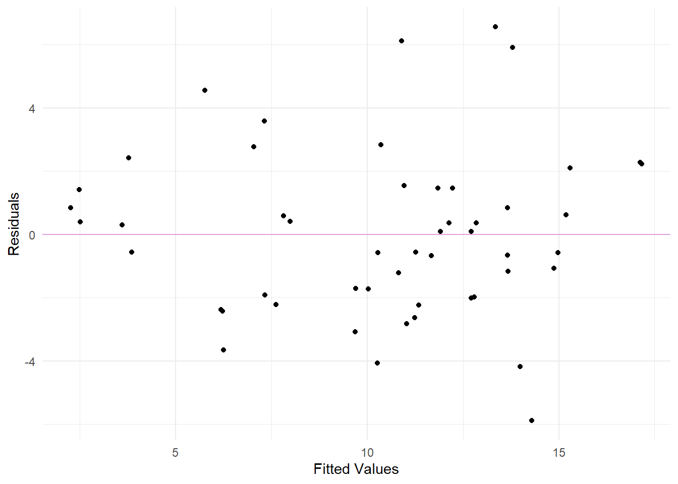
Residuals vs. Fits plot to examine non-linearity and constant variance assumptions.
From the above Residuals vs. Fits plot, there aren’t enough observations to make a sound conclusion. Linearity looks okay. Though, we should be a little worried about the constant variance assumption because it seems the points fan out from a thinner to a wider extent.
Normality Assumption.
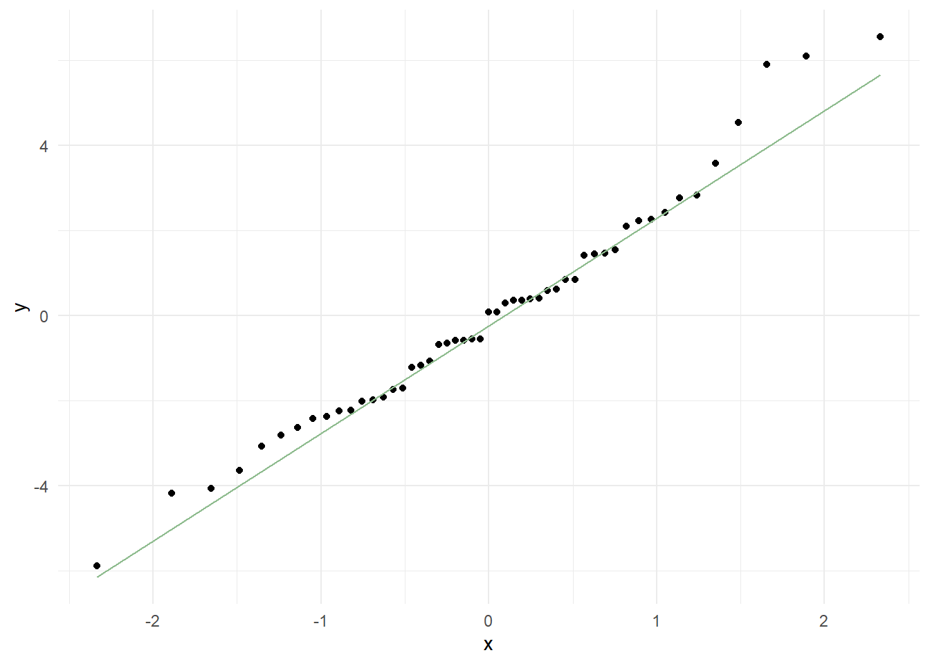
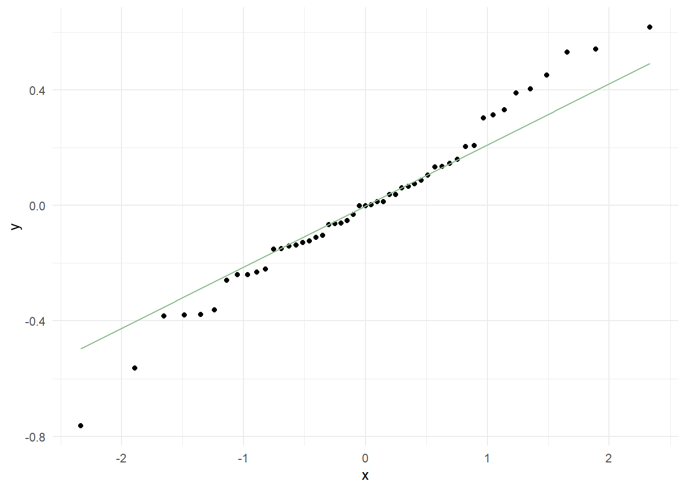
Q-Q plot to check normality of the residuals
There seems to be a little deviation for the upper plot, which suggests that there are outliers present. So, maybe we should use a different model.
d. Test the transformed model assumptions:
Here, we transform our linear regression by taking the \(\small\log\) of the predictor variable as follows.
modLog <- lm(log(sleep) ~ body + brain + lifespan +
gestation + predation + exposure +
danger, data = df)
Now, we test the model assumptions, similar to the above, for the transformed model.
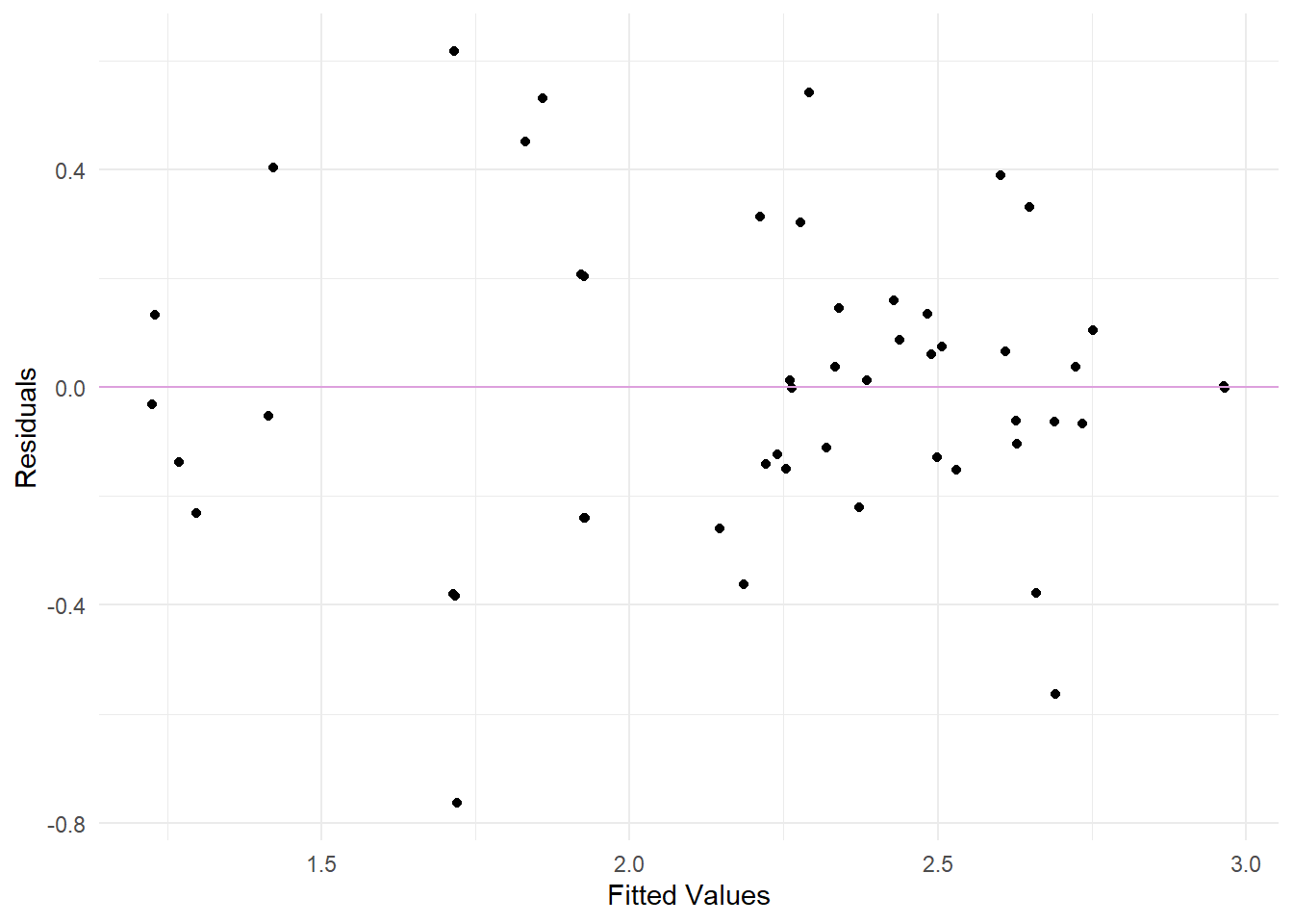
Residuals vs. Fits plot to examine non-linearity and constant variance assumptions and Q-Q plot to check normality of the residuals
Looking at the different plots, we can see that there are no significant improvements between the two models. Therefore, we will stick to the original squares regression model. Because we have a relatively small sample of 61 observations, we might violate some of the assumptions.
e. Interpret the Model’s Coefficients:
From above, we conclude that the original squares regression model is the better fit as opposed to a transformed model fit. Hence, we re-define our model as follows and evaluate its coefficients using tidy.
mod <- lm(sleep ~ body + brain + lifespan + gestation +
            predation + exposure + danger,
          data = df)
mod_table <- tidy(mod, conf.int = TRUE)
| term | estimate | std.error | statistic | p.value | conf.low | conf.high |
|---|---|---|---|---|---|---|
| (Intercept) | 16.6036994 | 1.0781762 | 15.399802 | 0.0000000 | 14.4293499 | 18.7780489 |
| body | -0.0016015 | 0.0014639 | -1.094016 | 0.2800386 | -0.0045537 | 0.0013507 |
| brain | 0.0023193 | 0.0016139 | 1.437113 | 0.1579230 | -0.0009354 | 0.0055740 |
| lifespan | -0.0398297 | 0.0353662 | -1.126209 | 0.2663232 | -0.1111523 | 0.0314930 |
| gestation | -0.0164652 | 0.0062143 | -2.649570 | 0.0112300 | -0.0289975 | -0.0039329 |
| predation | 2.3933611 | 0.9711013 | 2.464584 | 0.0177895 | 0.4349487 | 4.3517736 |
| exposure | 0.6329225 | 0.5585726 | 1.133107 | 0.2634478 | -0.4935465 | 1.7593916 |
| danger | -4.5085714 | 1.1861175 | -3.801117 | 0.0004491 | -6.9006054 | -2.1165374 |
The above summarizes information about the components of our final model, displaying each explanatory variables’ estimate, standard error, F Statistic, p-value, and the confidence interval bounds. Further assessing the model’s coefficients, we create a Forest-Plot to visualize the measures of effect of each explanatory variable and their confidence intervals.
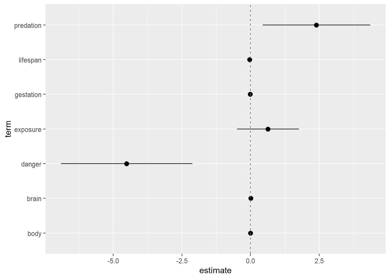
Forest Plot
It looks like there are two important variables: predation index and danger index. Based on the above, if we’re already including danger and predation, we don’t necessarily need to include the sleep exposure index.
f. The Final Model:
Here, we form our final model based on the above analysis of various linear model fits. We choose not to include the sleep exposure index because the danger index is a combination of the predation and exposure index. Therefore, the danger index consists of the information we might gain from exposure.
mod <- lm(sleep ~ body + brain + lifespan + gestation +
            predation + danger, data = df)

mod_table <- tidy(mod, conf.int = TRUE)| Term | Estimate | SE | Statistic | p-value | Lower Bound | Upper Bound |
|---|---|---|---|---|---|---|
| (Intercept) | 16.49 | 1.08 | 15.31 | 0.00 | 14.32 | 18.67 |
| body | 0.00 | 0.00 | -0.80 | 0.43 | 0.00 | 0.00 |
| brain | 0.00 | 0.00 | 1.14 | 0.26 | 0.00 | 0.00 |
| lifespan | -0.03 | 0.03 | -0.86 | 0.39 | -0.10 | 0.04 |
| gestation | -0.01 | 0.01 | -2.39 | 0.02 | -0.03 | 0.00 |
| predation | 2.18 | 0.95 | 2.28 | 0.03 | 0.25 | 4.10 |
| danger | -3.83 | 1.03 | -3.73 | 0.00 | -5.91 | -1.76 |
The variables body, brain, and lifespan have little impact on sleep duration when adjusting for body, brain, lifespan, gestation, predation, and danger, all with coefficients very close to \(\small 0\).
- A one day increase in lifespan yields an expected change in total sleep hours per day of \({\small -0.03}\) (95% CI: -0.10, 0.04) holding all other variables at constant.
- A one day increase in gestation time yields an expected change in total sleep hours per day of \({\small -0.01}\) (95% CI: -0.03, 0) holding all other variables at constant.
- A one unit change in predation index yields an expected change in total sleep of \({\small 2.18}\) (95% CI: 0.25, 4.1) hours per day holding all other variables constant.
- A one unit change in danger index yields an expected change in total sleep of \({\small -3.83}\) (95% CI: -5.91, -1.76) hours per day holding all other variables constant.
\[ \begin{gather} \color{darkgreen} \hat Y & \equiv {\small 16.49 - .001 X_1 + .002 X_2 - .03 X_3 - .01 X_4 + 2.18 X_5 - 3.83 X_6} & + {\large \varepsilon}_{\mathcal{\mid x,i}} \end{gather} \]
Checking Model Assumptions
| Assumptions | Checking Assumptions | Fixing Violated |
|---|---|---|
| Linearity | Residuals vs. Fits Plot | Transformations |
| Constant Variance | Residuals vs. Fits Plot | Weighted Least Squares |
| Normality | Q-Q Plot | Robust Regression |
| Correlated Error | Structure of the data | Generalized Least Squares |
| Unusual Observations | Calculated As |
|---|---|
| Leverage | \(\small\underbrace{H_{ii} = h_i}_{\text{diagonals of the hat matrix}}\) |
| Outliers | \(\underbrace{r_i = \frac{e_i}{s_e\sqrt{1 - h_i}}}_{\text{standardized residual}}\) |
| Influential Points | \(\underbrace{D_i = \frac{1}{p}r_i^2\frac{h_i}{1-{h_i}}}_{\text{Cook's Distance}}\) |