Sorting Algorithms
The sorting algorithms built in this lab are the Simple Bubble Sort, Merge Sort, and Insertion Sort. After making the algorithms, we ran them on different data points of sizes (50, 100, 200, 400, 800, 1000, 2000) and collected the number of steps for the data points in a text file. We then used the text file to plot the graphs for both algorithms.
Bubble Sort
Definition. Bubble sort checks and rechecks the relation between each component of the list. The method sorts the \(\mathrm{n}\) elements by linearly moving through the list where each pass completes \(\mathrm{n-1}\) comparisons and \(\mathrm{n-1}\) exchanges. After one pass, the largest integer-value should “bubble” up to the ArrayList’s high-indexed side –the operation repeats. After \(\mathrm{n-1}\) passes, the bubble sorting terminates.
a. The worst case has time complexity \(O(n^2)\); this occurs when the array is reverse sorted.
b. The best case has time complexity \(O(n)\). Bubble sort takes minimum time (Order of n) when elements are already sorted.
How does Bubble Sort act on the following list:
list XXX: 5 1 4 2 8\[ \small \begin{align} \begin{matrix} 5 & 1 & 4 & 2 & 8 \\ \bf{1} & \bf{5} & 4 & 2 & 8 \\ 1 & \bf{4} & \bf{5} & 2 & 8 \\ 1 & 4 & \bf{2} & \bf{5} & 8 \end{matrix} &\longrightarrow \begin{matrix} \bf{1} & \bf{4} & 2 & 5 & 8 \\ 1 & \bf{2} & \bf{4} & 5 & 8 \\1 & 2 & \bf{4} & \bf{5} & 8 \\1 & 2 & 4 & \bf{5} & \bf{8}\end{matrix} \longrightarrow \begin{matrix} \mathbf{1} & \mathbf{2} & 4 & 5 & 8 \\ 1 & \mathbf{2} & \mathbf{4} & 5 & 8 \\ 1 & 2 & \mathbf{4} & \mathbf{5} & 8 \\ 1 & 2 & 4 & \mathbf{5} & \mathbf{8} \end{matrix} \end{align} \]
Java Code
- Method sorts the elements by linearly moving through the list
- After a pass, the largest value “bubbles” up the ArrayList
- Bubble sorting repeats for (n-1) passes
// Bubble Sort Class

import java.util.ArrayList;

public class BubbleSort {

    // Used to count number of steps
    private static int Bcount = 0;

    // Getter
    public static int getBcount(){
        return Bcount;
    }

    // Setter
    public static void resetBcount(){
        Bcount = 0;
    }

    // Simple Bubble Sort -- O(n^2)
    // Requires isLessThan from interface Relateable
    // Uses a generic class T which extends Relateable
    public static <T extends Relateable> ArrayList<T> Bubble(ArrayList<T>  A){

        // Depth of split levels:
        // number of times n can be halved while value is greater than 1
        if (A.size() <= 1) return A;

        // Each pass of the bubbling phase performs n-1 comparisons and n-1 exchanges
        // After n-1 passes, the method terminates
        for(int passes = 0; passes < A.size()-1; passes++){

            for(int index = 0; index < A.size() - passes - 1; index++){

                Bcount++;
                if (A.get(index).isLessThan(A.get(index + 1))){
                    T temp = A.get(index + 1);
                    A.set(index + 1, A.get(index));
                    A.set(index, temp);
                }

            }
        }

        return A;
    }

}
Execution Times
| DataPoints | Steps |
|---|---|
| 50 | 1225 |
| 100 | 4950 |
| 200 | 19900 |
| 400 | 79800 |
| 800 | 319600 |
| 1000 | 499500 |
| 2000 | 1999000 |
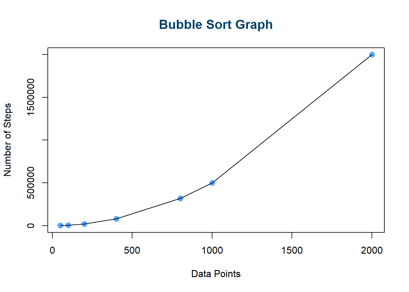
From the above execution times and graph, we can see that as the number of data points \(\mathrm{n}\) increases, the number of steps it takes to complete the bubble sort increases exponentially. In big-O notation, the Simple Bubble Sort Method for sorting \(\mathrm{n}\) elements of an array is \(O\mathbf{(n^2)}\); hence, the algorithm has a run time that grows quadratically as the input (data points) size grows.
Merge Sort
Definition. MergeSort is a recursive sorting technique that recursively splits, sorts, and reconstructs the data. This method recursively divides the data into two unsorted lists, sorts the two lists, and then merges the two sorted lists. In big-O notation, we have a time execution of \(O(\mathrm{n \log{n}})\); hence, the search algorithm has a run time that grows logarithmically as the input size grows. Similar to MergeSort, binary search trees are nonlinear structures that execute in logarithmic time.
a. Merge Sort is a recursive algorithm and time complexity can be expressed by \(\theta(n\log n)\).
b. Time complexity of Merge Sort is \(\theta(n\log n)\) in all 3 cases (worst, average and best) as merge sort always divides the array into two halves and takes linear time to merge two halves.
Java Code
- Break the whole array down into two subarrays
- Sort the left half of the array (recursively)
- Sort the right half of the array (recursively)
- Merge the solutions
// Merge Sort Class

import java.util.ArrayList;

public class MergeSort {

    private static int Mcount = 0;

    // Getter
    public static int getMcount(){
        return Mcount;
    }

    // Merge Sort --  O(nlog2(n))
    // Requires isLessthan from interface Relateable
    // Uses a generic T which extends Relateable

    // Public signature
    // This nonrecursive part takes care of small lists
    public static <T extends Relateable> ArrayList<T> MergeSort(ArrayList<T> A){
        Mcount++;
        if (A.size() <= 1) {return A;}
        return RMergeSort(A);
    }

    // Recursive RMergeSort method--
    // Private signature for the recursive part
    // Requires isLessthan from interface Relateable
    // Uses a generic T which extends Relateable
    private static <T extends Relateable> ArrayList<T> RMergeSort(ArrayList<T> A){

        // Middle index to divide the ArrayList into two halves
        int mid = A.size() / 2;

        // Create two temporary arrays:
        ArrayList<T> B = new ArrayList<>(); // first half
        ArrayList<T> C = new ArrayList<>(); // second half

        for(int i = 0; i < mid; i++) {
            B.add(A.get(i));
        }
        for(int i = mid; i < A.size(); i++) {
            C.add(A.get(i));
        }

        // Call mergeSort for first half:
        B = MergeSort(B);

        // Call mergeSort for second half:
        C = MergeSort(C);

        // Merge the two halves sorted:
        return Merge(B,C);
    }

    // Merge method-- merge A and B routine
    // Requires isLessthan from interface Relateable
    // Uses a generic T which extends Relateable
    private static <T extends Relateable> ArrayList<T> Merge(ArrayList<T> A, ArrayList<T> B){
        ArrayList<T> C = new ArrayList<>();
        int j = 0;
        int k = 0;

        // Compares the elements of both sub-arrays one by one
        while(j < A.size() && k < B.size()) {
            if (A.get(j).isLessThan(B.get(k))) {
                C.add(A.get(j));
                j++;
            }
            else{
                C.add(B.get(k));
                k++;
            }
        }
        while(j < A.size()) {
            C.add(A.get(j));
            j++;
        }
        while(k < B.size()) {
            C.add(B.get(k));
            k++;
        }

        return C; // sorted array
    }

}
Execution Times
| DataPoints | Steps |
|---|---|
| 50 | 99 |
| 100 | 199 |
| 200 | 399 |
| 400 | 799 |
| 800 | 1599 |
| 1000 | 1999 |
| 2000 | 3999 |
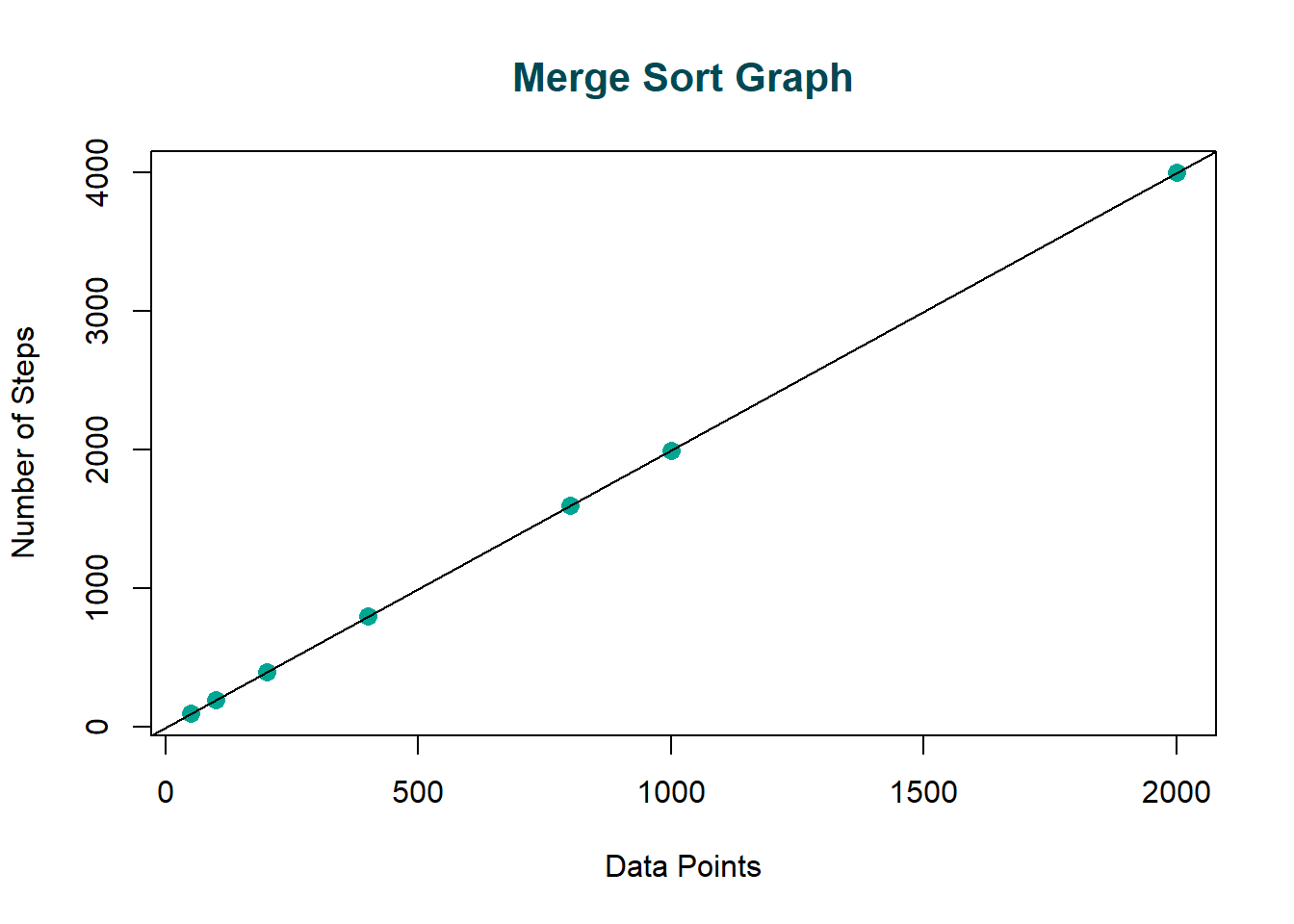
Each value \(\mathrm{n}\) in the data set must be sorted into a temporary array, allotted once before every single merge; therefore, we have \(O(\mathrm{n})\) compares over all the merges. From the above execution times and graph, we can see that as the number of data points \(\mathrm{n}\) increases, the number of steps it takes to complete the bubble sort increases logarithmically. In big-O notation, since there are \(\mathrm{\log{2}n}\) split levels, we have a time execution of \(O(\mathrm{n \log{n}})\); hence, the search algorithm has a run time that grows logarithmically as the input size grows.
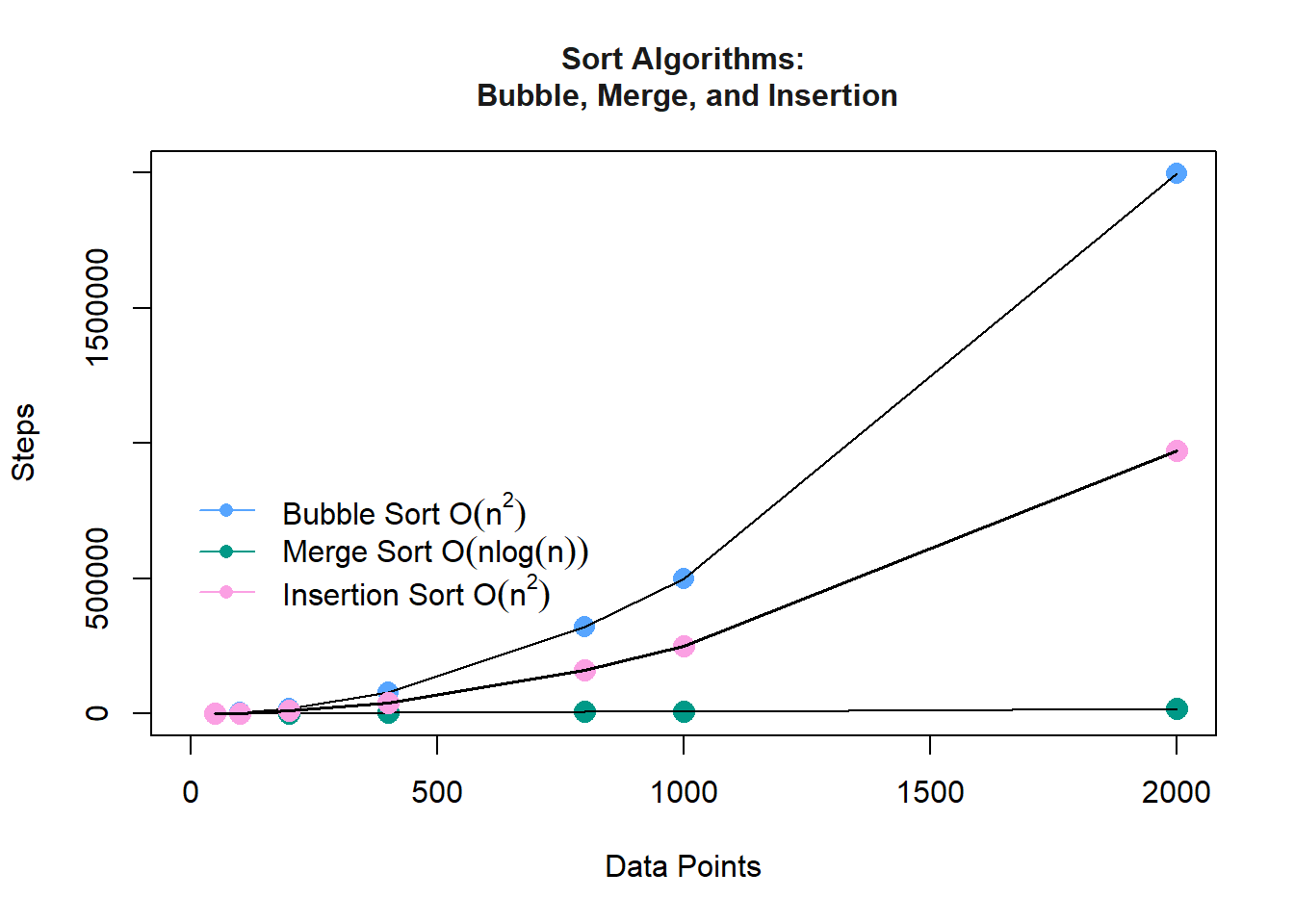
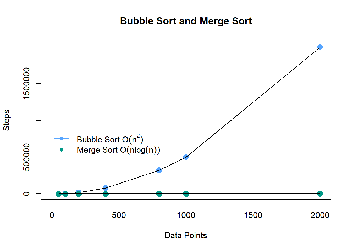
Comparing Sort Algorithms. From the graph below, we can see that the number of steps to execute the Merge Sort method is significantly lower than the number of steps to execute the Bubble Sort method; hence, the Merge Sort is faster and more efficient than the Bubble Sort.
Insertion Sort
Definition. a Java sorting method where the sorted values locate to the low end of the array, and the unsorted values locate to the high end.
a. total of \(n-1\) passes over the array, with a new unsorted value inserted each time
b. expected running time is \(\mathbb{O}\left(n^2\right)\) compares and data movements –most compares will lead to movement of a data value
c. best case running time performance is \(\mathbb{O}\left(n\right)\) comparisons –occurs for no movements of data within the array; therefore, it’s best to implement insertion sort on data that is nearly ordered
On average, it is \(i/2\) positions out of order
| \(0 \;\) | \(1 \;\) | \(\dots\) | \(i-1\) | \(i\;\) | \(\dots\) | \(n-1\) |
And since this is done from \(1\) to \(n-1\), then we have the total cost as
\[\sum^{n-1}_{i=1} \frac{i}{2} = \frac{n(n+1)}{4}\]
Therefore, the average case running time of insertion sort is \(\mathbf{O(n^2)}\)
Show how Insertion Sort acts on the following List:
list X: 7 5 4 6 8 2\[ \begin{align} \begin{matrix} \mathbf{7} & 5 & 4 & 6 & 8 & 2 \end{matrix} \\ \begin{matrix} \mathbf{5} & \mathbf{7} & 4 & 6 & 8 & 2 \end{matrix} \\ \begin{matrix} \mathbf{4} & \mathbf{5} & \mathbf{7} & 6 & 8 & 2 \end{matrix} \\ \begin{matrix} \mathbf{4} & \mathbf{5} & \mathbf{6} & \mathbf{7} & 8 & 2 \end{matrix} \\ \begin{matrix} \mathbf{4} & \mathbf{5} & \mathbf{6} & \mathbf{7} & \mathbf{8} & 2 \end{matrix} \\ \begin{matrix} \mathbf{2} & \mathbf{4} & \mathbf{5} & \mathbf{6} & \mathbf{7} & \mathbf{8} \end{matrix} \end{align} \]
Java Code
a generic type that extends the interface Relateable
- create a LinkedList
- initialize ICount
- walk down ArrayList and insert each element into sorted LinkedList
- repackage and return ArrayList
- method to insert a new element myObj into a sorted LinkedList
- use a loop to traverse LinkedList
- begin with first element (smallest T) and find where myObj should go
- debugging tool and method to dump out content in LinkedList
import java.util.LinkedList;
import java.util.ListIterator;
import java.util.ArrayList;

public class InsertionSort {

  private static int ICount;
  public static int getICount(){
    return ICount; }

  // a generic type that extends the interface Relateable
  public static <T extends Relateable> ArrayList<T> InsertionSort(ArrayList<T> myAL){

    // create a LinkedList
    LinkedList<T> mylist = new LinkedList<T>();

    // initialize ICount
    ICount = 0;

    // walk down ArrayList and insert each into sorted LinkedList
    for(T XXX: myAL){
      insert(mylist, XXX); }

    // repackage myAL from the LinkedList and return it
    return myAL; }

  // insert new element myObj into sorted LinkedList
  public static  <T extends Relateable> void insert(LinkedList<T> mylist, T myObj) {

    // if myList is empty, add myObj and return
    if (mylist.isEmpty()) {
      ICount++;
      mylist.add(myObj);
      return; }

    // use a loop to traverse LinkedList
    // begin with first element (smallest T) and find where myObj goes
    ListIterator current = mylist.listIterator();
    while(current.hasNext()){

      // get value and advance iterator
      ICount++;
      T temp = (T)(current.next());

      // figure out out if I should add now or not
      if (temp.isLessThan(myObj)){
        continue; }

      // add on the list iterator but where?
      else{
        current.add(myObj);
        return; }}

    // **************************
    // if we get here, then I should add myObj at the end of the list
    // ICount++;
    // mylist.addLast(myObj);
    // return; }

  // method to dump out content in LinkedList
  // debugging tool
  private static <T> void dump (LinkedList<T> mylist){
    ListIterator<T> current = mylist.listIterator();
    for(int i=0; i< Math.min(15, mylist.size()); i++){
      System.out.println((T)(current.next()).toString()); }}

  }
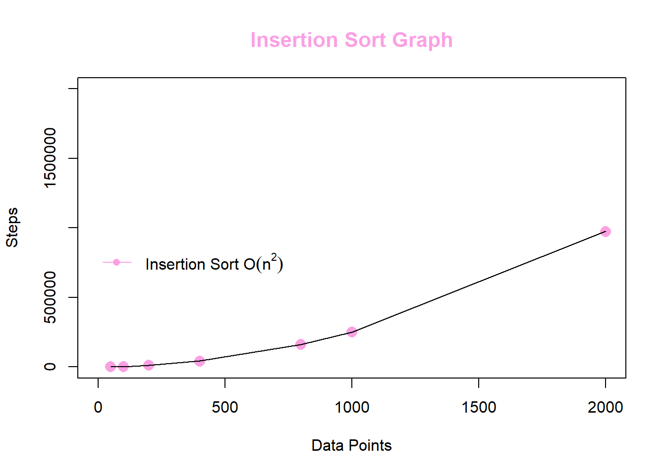
Execution Times
At the worst case scenario for the algorithm, the whole array is descending. This is because in each iteration, we’ll have to move the whole sorted list by 1, which is \(O(n)\). We have to do this for each element in every array, which means it’s going to be bounded by \(O(n^2)\).
| DataPoints | Steps |
|---|---|
| 50 | 671 |
| 100 | 2395 |
| 200 | 9743 |
| 400 | 39658 |
| 800 | 161494 |
| 1000 | 251346 |
| 2000 | 974151 |
Conclusion
From the graph below, we can see that the number of steps to execute the Merge Sort method is significantly lower than the number of steps to execute the Bubble Sort method; hence, the Merge Sort is faster and more efficient than the Bubble Sort.